New tools for visualising and explaining multivariate spatio-temporal data
Monash University, Australia
Apr 17, 2023
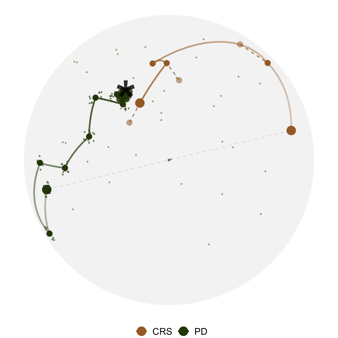
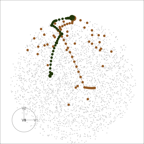
Projection pursuit for dimension reduction
Visualise the projection matrix space
Data: \(\mathbf{X}_{n \times p}\);
Projection matrix: \(\mathbf{A}_{p\times d}\)
Projection: \(\mathbf{Y}_{n \times d} = \mathbf{X} \cdot \mathbf{A}\)
Index function \(f: \mathbb{R}^{n \times d} \mapsto \mathbb{R}\)
Optimisation: \[\arg \max_{\mathbf{A}} f(\mathbf{X} \cdot \mathbf{A}) ~~~ s.t. ~~~ \mathbf{A}^{\prime} \mathbf{A} = I_d\]
Simulation:
- simulated 5D data project to 1D
- two optimisers

Visualise the projection matrix space

Visualise the projection matrix space
Motivation
![]()
![]()
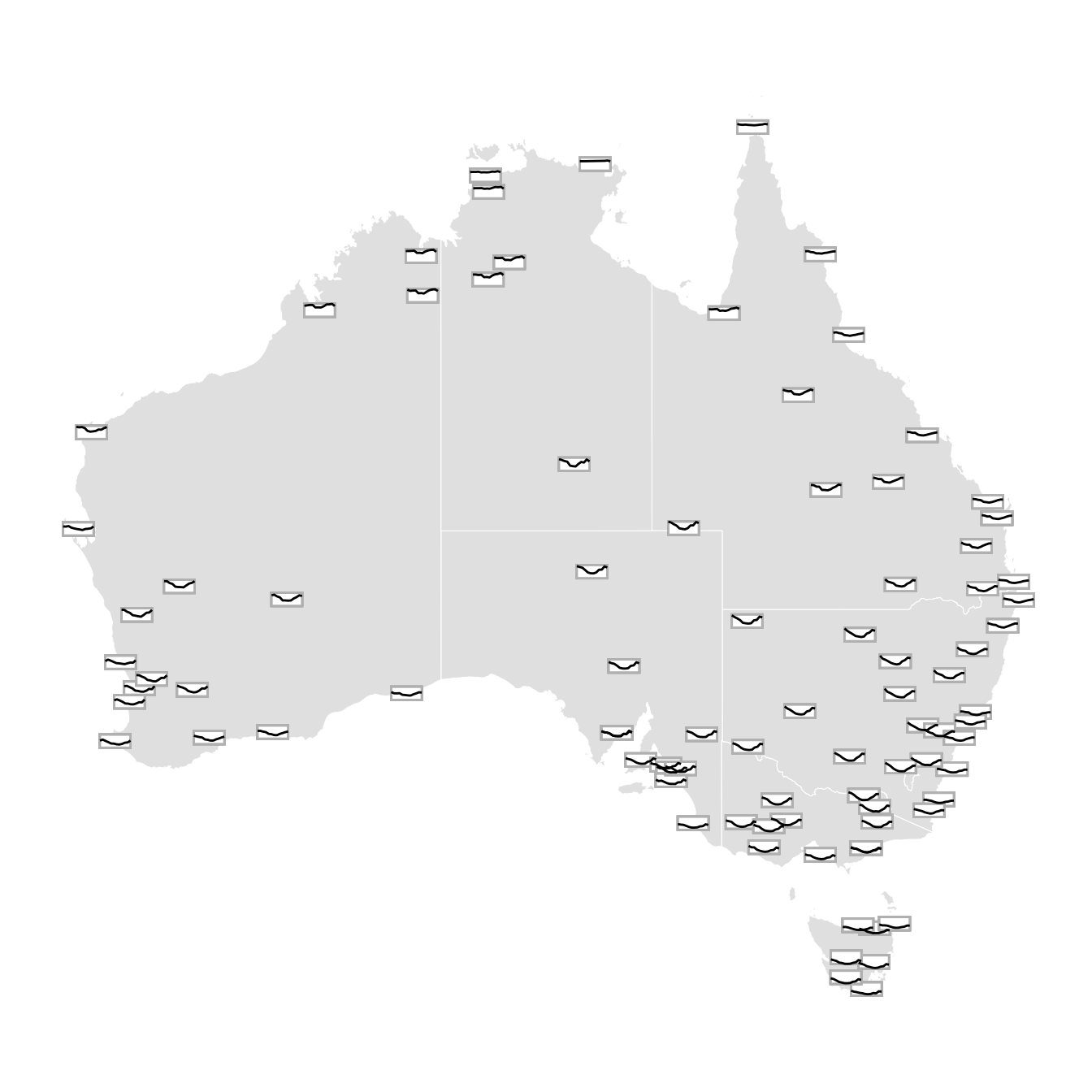
Australian weather station data
# A tibble: 88 × 6
   id            lat  long  elev name              wmo_id
   <chr>       <dbl> <dbl> <dbl> <chr>              <dbl>
 1 ASN00001006 -15.5  128.   3.8 wyndham aero       95214
 2 ASN00002032 -17.0  128. 203   warmun             94213
 3 ASN00003080 -17.6  124.  77.5 curtin aero        94204
 4 ASN00005007 -22.2  114.   5   learmonth airport  94302
 5 ASN00006044 -25.9  114.   9   denham             94402
 6 ASN00007600 -28.1  118. 407   mount magnet aero  94429
 7 ASN00008296 -29.2  116. 271.  morawa airport     94417
 8 ASN00009114 -31.0  115.   4   lancelin           95606
 9 ASN00009240 -32.0  116. 384   bickley            95610
10 ASN00009542 -33.7  122. 142   esperance aero     95638
# … with 78 more rows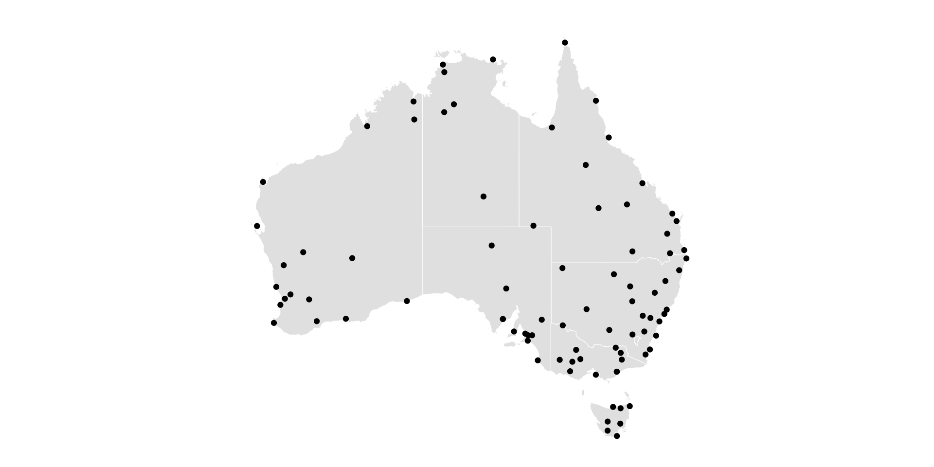
# A tibble: 32,208 × 5
   id          date        prcp  tmax  tmin
   <chr>       <date>     <dbl> <dbl> <dbl>
 1 ASN00001006 2020-01-01   164  38.3  25.3
 2 ASN00001006 2020-01-02     0  40.6  30.5
 3 ASN00001006 2020-01-03    16  39.7  27.2
 4 ASN00001006 2020-01-04     0  38.2  27.3
 5 ASN00001006 2020-01-05     2  39.3  26.7
 6 ASN00001006 2020-01-06    60  32.9  25.6
 7 ASN00001006 2020-01-07   146  34.1  25.5
 8 ASN00001006 2020-01-08    40  36.6  26.2
 9 ASN00001006 2020-01-09     0  38.2  27.6
10 ASN00001006 2020-01-10     0  38.9  29.7
# … with 32,198 more rows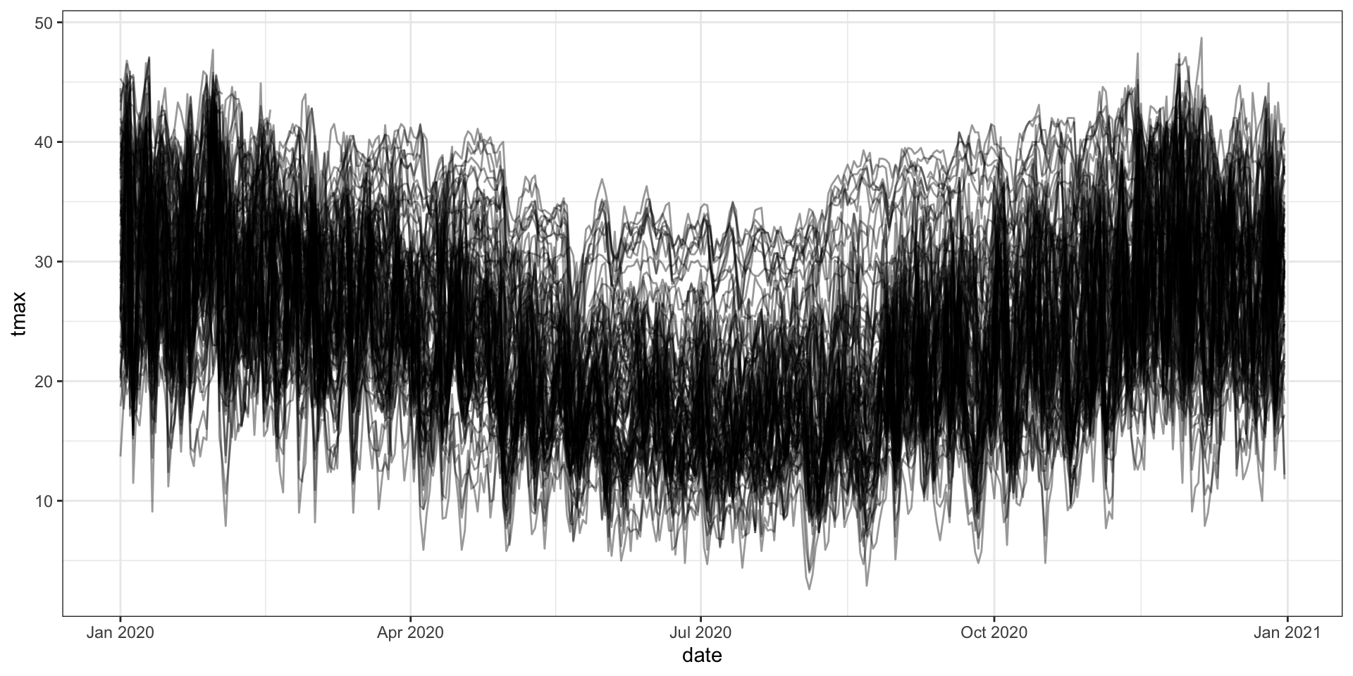
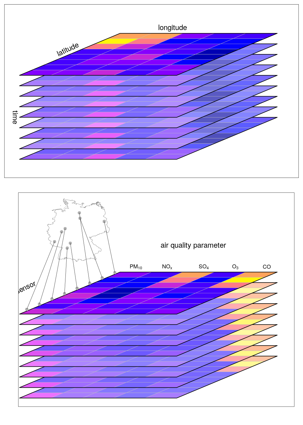
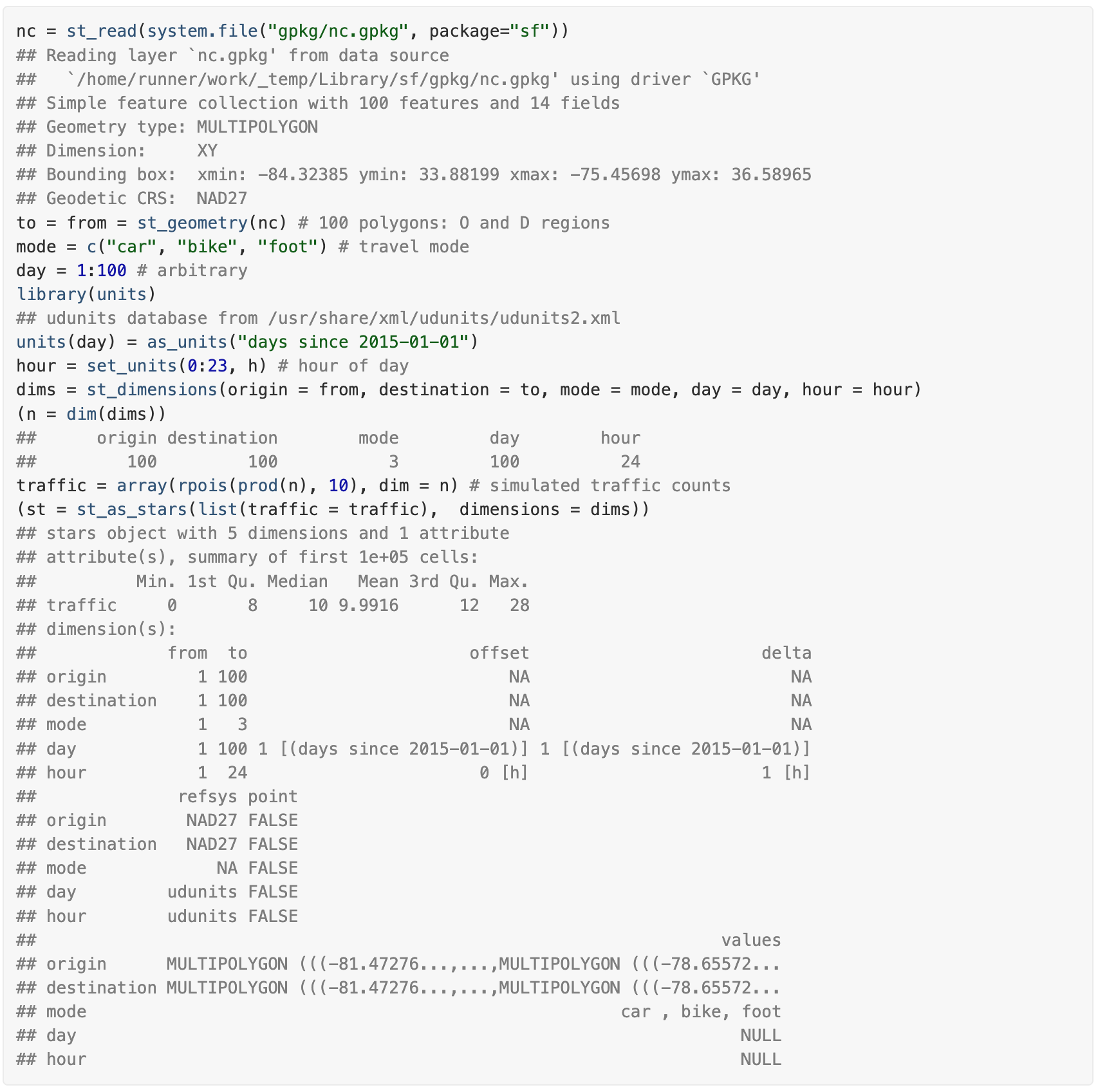
What’s available for spatio-temporal data? - stars
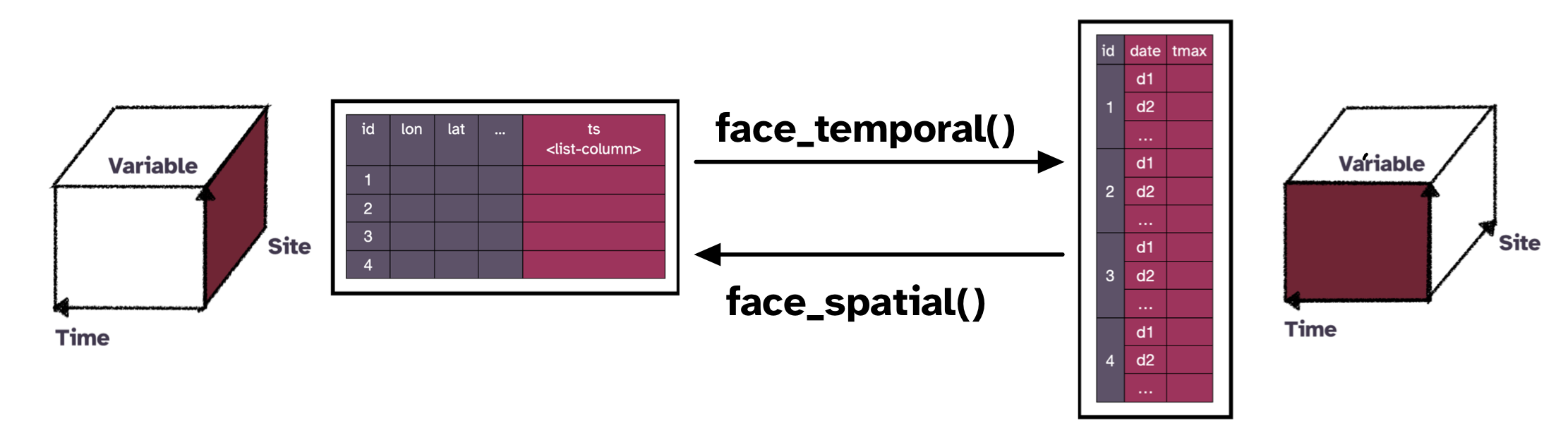
Cubble: a spatio-temporal vector data structure

Cubble: a spatio-temporal vector data structure
Cubble is a nested object built on tibble that allow easy pivoting between spatial and temporal form.
Why do you need a glyph map?

Why do you need a glyph map?

Glyph map transformation
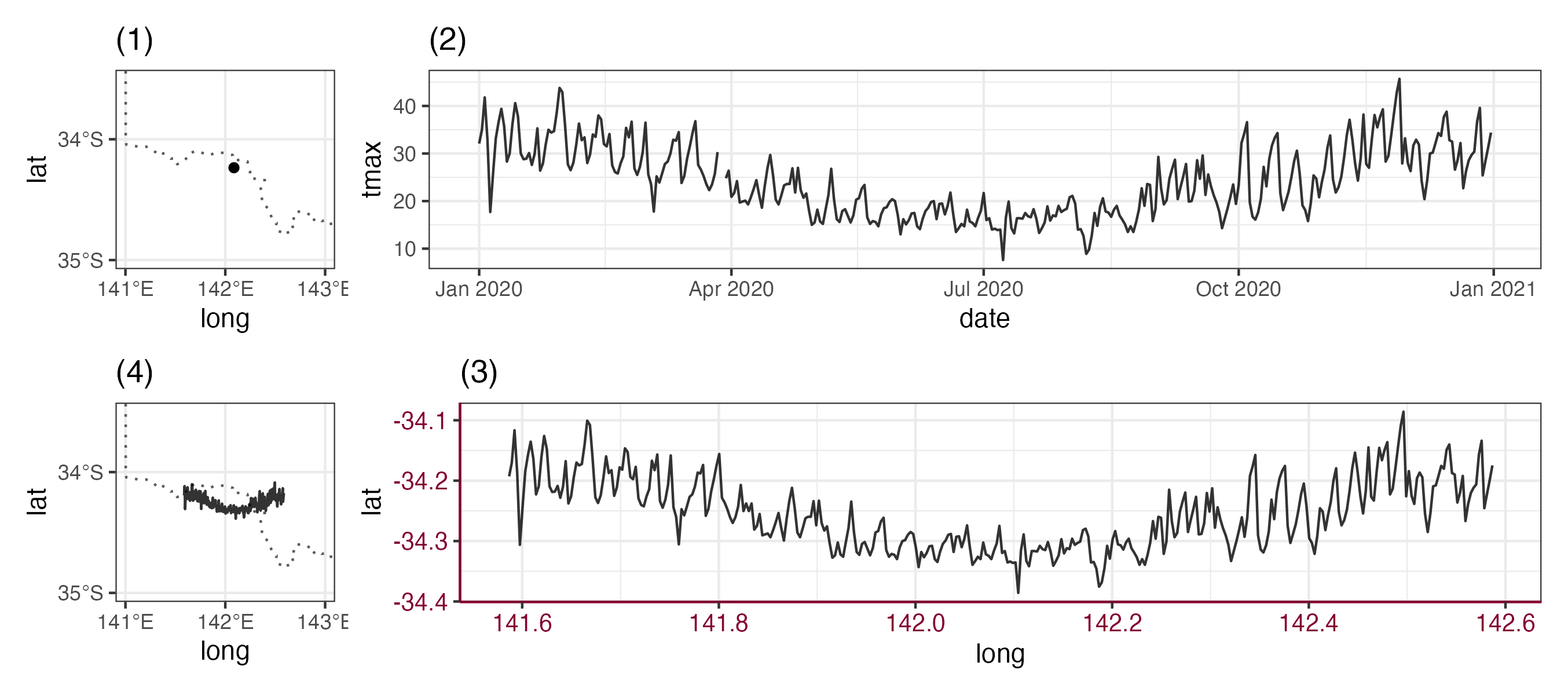
Avg. max. temperature on the map
cb <- as_cubble(
  list(spatial = stations, temporal = ts),
  key = id, index = date, coords = c(long, lat)
)

cb_glyph <- cb %>%
  face_temporal() %>%
  group_by(month = lubridate::month(date)) %>%
  summarise(tmax = mean(tmax, na.rm = TRUE)) %>%
  unfold(long, lat)

cb_glyph %>%
  ggplot(aes(x_major = long, x_minor = month,
             y_major = lat, y_minor = tmax)) +
  geom_sf(data = oz_simp, fill = "grey90",
          color = "white", inherit.aes = FALSE) +
  geom_glyph_box(width = 1.3, height = 0.5) +
  geom_glyph(width = 1.3, height = 0.5) +
  ggthemes::theme_map()